This paper is available on arxiv under CC 4.0 license.
Authors:
(1) Amit Kumar Chatterjee, Yukawa Institute for Theoretical Physics, Kyoto University & Department of Physics, Ramakrishna Mission Vidyamandira;
(2) Satoshi Takada, Department of Mechanical Systems Engineering and Institute of Engineering;
(3) Hisao Hayakawa, Yukawa Institute for Theoretical Physics, Kyoto University.
Table of Links
- Introduction
- Model and Protocol
- Different Regimes in d˜− Γ˜ Plain and Multiple QMPE
- QMPE in Region (d): Second-order Ep
- QMPE in Region (a1): Oscillations
- Summary
- Appendix A: Eigenvectors of L in region (d)
- Appendix B: Eigenvectors of L in region (a1)
- Appendix C: QMPE in region (b): purely exponential relaxation
- Appendix D: QMPE in region (e): 3rd order EP
- References
V. QMPE IN REGION (a1): OSCILLATIONS
In this section, we explore QMPE in region (a1) of Hatano’s model which contains complex eigenvalues with both non-zero real and imaginary parts. The eigenvalues are non-degenerate and they are denoted by 0, λ2, λ3 = λre+iλim, λ4 = λre−iλim, where the subscripts re and im correspond to real and imaginary parts, respectively. In addition, the eigenvalues satisfy the relation 0 < λ2 < λre meaning λ2 is the slowest relaxation mode. In contrast to the nontrivial approximate diagonalization [Eqs. (10)- (11)] for second-order EP in Sec. IV, here the complete diagonalization can be obtained through the usual method

A. Density matrix elements
The the individual density matrix elements ρj (t) (j = 1, 2, 3, 4) are given by

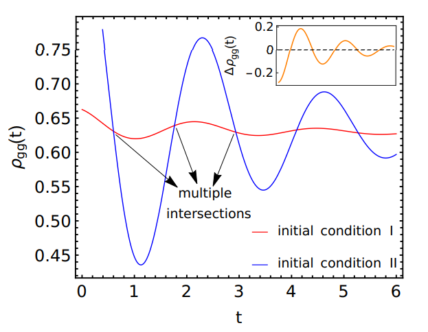
To discuss QMPE in the density matrix, let us focus on the ground state probability i.e. ρgg(t). Of course, there is no algebraic time dependence in the relaxation observed in Sec. IV. Rather, the interesting part of the relaxation in region (a1) originates from the complex nature of the eigenvalues and the corresponding coefficients ak in Eq. (27). Specifically, we have found that a3 and a4 are complex conjugates of each other, they take the forms a3 = are + iaim and a4 = are − iaim. Using such expressions, we obtain the following formula for ρgg(t):

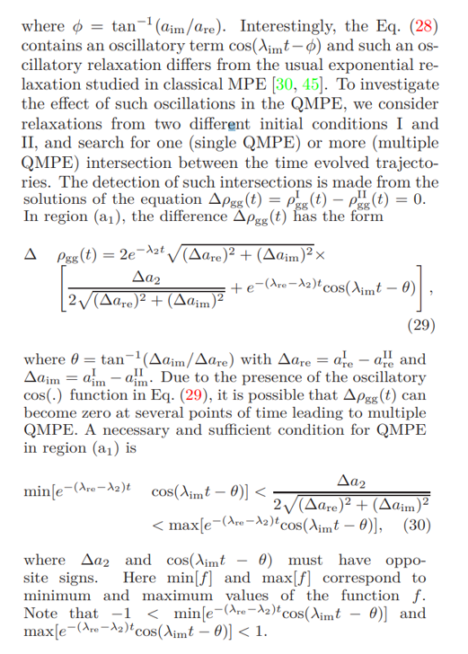
In Fig. 7 we present an example of multiple QMPE in the ground state density matrix element ρgg(t), where we have chosen parameters that satisfy the QMPE criteria Eq. (30) for region (a1). We observe that the two copies I and II relax in oscillatory manner and intersect each other multiple times. The inset explicitly shows that the difference between the two copies ∆ρgg(t) intersects zero multiple times, confirming the multiple QMPE. Comparing Fig. 3(a) [region (d)] with the inset of Fig. 7 [region (a1)], we understand that the number of intersections in region (a1) is not restricted to two as in region (d). Therefore, in region (a1) one can have many more intersections and higher order QMPE compared to the maximum double QMPE in the region (d). Since the amplitudes of the oscillations can be controlled by tuning the initial driving strengths ˜dI and ˜dII, complex eigenvalues seem to be useful to obtain multiple intersections and thereby multiple QMPE. It would be important in the future to find the exact number of solutions to ∆ρgg(t) = 0 either analytically or numerically.
B. Energy
The formal expression for average energy E(t) is given by Eq. (18). In the previous Sec. IV, we have already shown that QMPE in ground state probability does not necessarily imply QMPE in energy, in general. However, it is possible to find control parameters that can give rise to QMPE in both observables, although the intersection time(s) are generally different. Following the same path, we would like to see if E(t) shows multiple QMPE for the same set of parameters used to achieve multiple QMPE
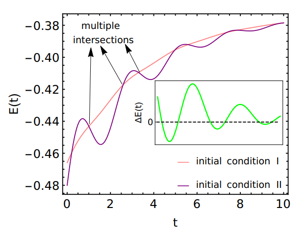
for ρgg(t) in Fig. 7. Indeed, Fig. 8 exhibits multiple intersections between time evolved copies of energies starting from I and II, both relaxing towards the same final energy. The inset of Fig. 8 alternatively demonstrates the multiple QMPE through multiple intersections of the energy difference ∆E(t) = EI(t)−EII(t) with zero, remarkably different from Fig. 3(b) with a maximum of two such intersections in region (d).
C. von Neumann entropy
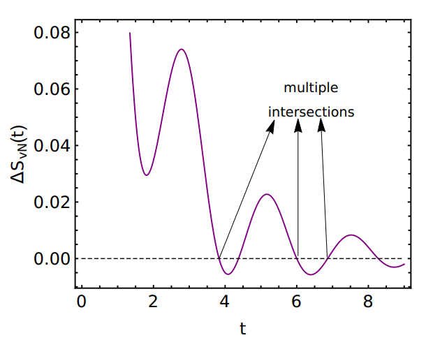
Next we consider the von Neumann entropy SvN(t) [Eq. (22)]. To observe QMPE in SvN(t), we consider the intersection times for the entropy difference between two copies ∆SvN(t) = S I vN − S II vN. In Fig. 9, we present the behavior of ∆SvN(t) for the same set of parameter values used in Figs. 7 and 8. Indeed, we observe that ∆SvN(t) intersects zero multiple times showing the existence of multiple QMPE in the von Neumann entropy.
D. Temperature
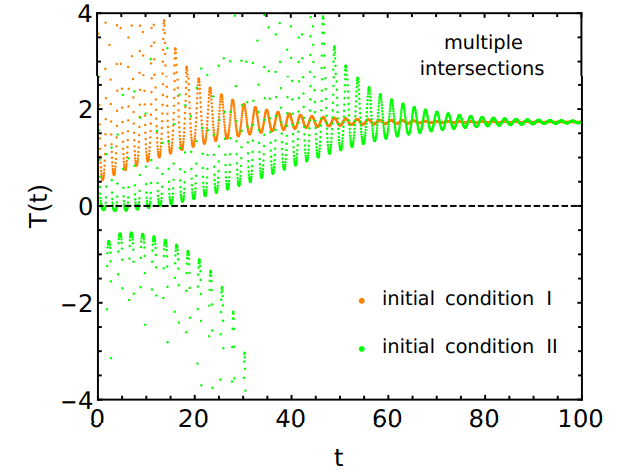
Here, we study the thermal QMPE in region (a1) using the system temperature defined in Eq. (23). In Fig. 10, we present the time evolution of the temperatures of two copies I and II, one initially hotter than the other. It is fascinating that the temperatures of both the copies relax in oscillatory manner towards the same steady state temperature and during the relaxations, they intersect each other multiple times, leading to multiple thermal QMPE. This, in turn, implies that the hotter and colder
copies reverse their identities multiple times (after each intersection the previous hotter copy turns into colder copy and remains so until the next intersection). Such oscillatory multiple thermal QMPE is observed here for the first time in quantum systems (as far as our knowledge is concerned), although multiple thermal MPE in classical inertial suspensions has already been reported [42]. The physical interpretation and utility of multiple thermal QMPE have to be explored in future in more details. Note that we have used the same parameter set for multiple thermal QMPE as in Figs. 7-9. Similar to Ref. [65], here also we observe negative temperature [114– 118] in the early stage of relaxation. This is due to nonmonotonic natures of energy and entropy as functions of time. However, it is satisfying that even if we neglect such initial negative temperatures, we observe multiple QMPE at later times of the relaxation process where the temperatures of both the copies remain positive.
E. Kullback-Leibler divergence
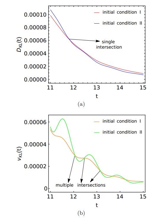
In this subsection we explore the QMPE in KL divergence defined in Eq. (24). Since we have been able to obtain multiple QMPE in region (a1) in all other observables considered here, it is natural to ask about the possibility of multiple QMPE in DKL(t) as well. However, we have found that the KL divergence does not show any intersection between two copies I and II for the same parameter values used in Figs. 7-10. Therefore, we have to use different values of the initial drives (still within the fixed dissipation protocol) to achieve QMPE in DKL(t), presented in Fig. 11(a). Intriguingly, we have only observed single intersection between the two time
evolved copies, resulting in single QMPE in KL divergence. This means that once the initially higher distant copy intersects the initially lower distant copy producing QMPE, thereafter the new lower distant copy (that was initially higher distant) remains closer to the steady state for the rest of the relaxation process. In fact, for all other parameter sets that we have checked, we could not find multiple QMPE in DKL(t). The proof of the possibility or impossibility of multiple QMPE in KL divergence in presence of complex eigenvalues remains unsolved and could be an important question to investigate later.
In this scenario, it would be interesting to examine the corresponding behaviors of the speeds vKL(t) [Eq. (25)] of the two copies I and II. In Fig. 11(b), we present the time evolution of speeds for the same set of parameters that gave rise to single QMPE in DKL(t). It is fascinating to observe that the speeds, unlike the distances, intersect each other multiple times producing multiple QMPE. The first intersection between the speeds of the two copies [Fig. 11(b)] shows a time lag in comparison to the intersection between distances of the same copies [Fig. 11(a)]. Such a time lag between the QMPE in KL divergence and the speed is in agreement with the observation in region (d) [Fig. 6]. However, contrary to single QMPE in vKL(t) in region (d), we have obtained multiple QMPE in the speed in region (a1). The contrasting behavior of single QMPE in DKL(t) and multiple QMPE in vKL(t) imply that the initially higher distant copy that becomes lower distant after the intersection in distances, can remain at lower distance even if its speed sometimes become smaller than the speed of the current higher distant copy. This is interesting because the system almost
behaves like an intelligent and efficient runner in a race who knows how to adjust the speed (i.e. sometimes running faster and sometimes running slower than the people behind) and still remains in the first position to finish the race.

