Multiple Quantum Mpemba Effect: Exceptional Points and Oscillations: Appendix D: QMPE in Region (e)

Table of Links

• Introduction
• Model and Protocol
• Different Regimes in d˜− Γ˜ Plain and Multiple QMPE
• QMPE in Region (d): Second-order Ep
• QMPE in Region (a1): Oscillations
• Summary
• Appendix A: Eigenvectors of L in region (d)
• Appendix B: Eigenvectors of L in region (a1)
• Appendix C: QMPE in region (b): purely exponential relaxation
• Appendix D: QMPE in region (e): 3rd order EP
• References

Appendix D: QMPE in region (e): 3rd order EP

The region (e) in the (d,˜ Γ) plane of Hatano’s model is composed of a single point

It is a third order EP where all the non-zero eigenvalues become equal and their eigenvectors coalesce. Since this is a single point with fixed values of ˜d and Γ, the right eigenvectors are explicitly given by

Of course |r1i and hℓ1| have same expressions both in Eqs. (3) and (D2). The left eigenvectors are

) The non-zero eigenvalue of the Lindbladian [Eq. (2)] in region (e) is −iλ = −i4√ 3. Importantly, as a consequence of the 3rd order EP, we can only achieve an approximately diagonal form i.e. Jordan normal form LbJn leading to the equation

Due to the off-diagonal nonzero defects in Eq. (D5), the time evolution of density matrix elements and other observables pick up additional algebraic terms in time.

1. Density matrix elements

In region (e), the density matrix elements have the expressions below

In Fig. 15(a), we present existence of t˜+ and t˜− as function of the control parameters ˜dI and ˜dII using the fixed dissipation protocol. The solutions’ surfaces in Fig. 15(a) reveal that there are regions where only one of the solutions t˜+ or t˜− exist leading to single QMPE, and in other regions both the solutions exist resulting in double QMPE. Particularly, lower values of ˜dI and ˜dII correspond to single intersection time solution and therefore single QMPE. To understand the behaviors of t˜+,− more clearly, we fix ˜dI and display t˜+,− as functions of ˜dII in Fig. 15(b). The

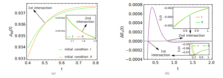
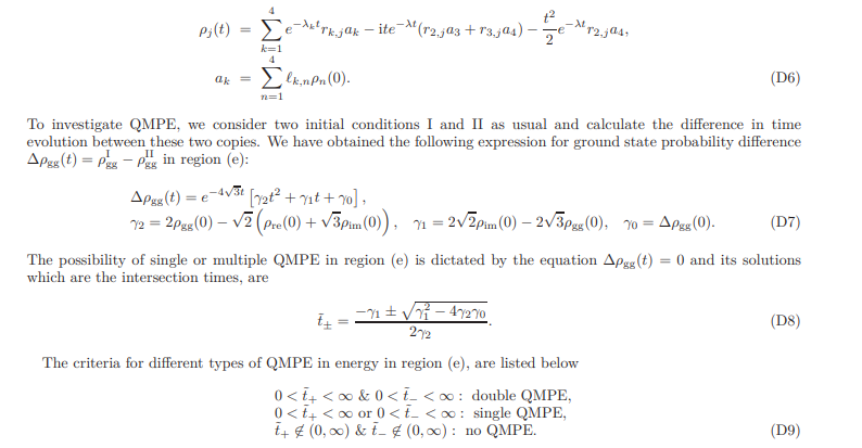
Fig. 15(b) shows that the two branches t˜+ and t˜− interchange as ˜dI < ˜dII. More specifically, for ˜dI > ˜dII we have t˜+ > t˜− and for ˜dI < ˜dII we have t˜+ < t˜−. The underlying reason is that the discriminant p γ 2 1 − 4γ2γ0 in Eq. (D8) is proportional to sign of ( ˜dI − ˜dII). Thus the two intersection times interchange their roles by changing the sign accompanying the discriminant as we go from ˜dI > ˜dII to ˜dI < ˜dII. The Fig. 16(a) demonstrates an explicit example of double QMPE in ground state probability in region (e). Like other regions, here also the second intersection (shown in the inset of Fig. 16(a)) is much feeble in comparison to the first intersection.

2. Average energy

For the same parameters used to obtain QMPE for ρgg(t) in Fig. 16(a), we would like to examine the possibility of QMPE in average energy E(t). Indeed, we observe in Fig. 16(b) that energy also exhibits double QMPE, marked by the twice intersection of zero by the energy difference ∆E(t) between the two copies. The insets of Fig. 16(b) shows separately the two intersections in the time evolution of the energies for the two copies. The second intersection is much weaker in magnitude compared to the first intersection just like the case of ground state probability. Note that the first intersection between the energies of I and II occur after they overshoot their steady state value which they reach during some early time of the relaxation process.

3. von Neumann entropy

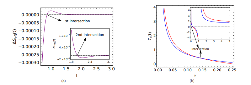
Here we investigate the von Neumann entropy SvN(t), starting from two copies I and II. We use same parameters that have produced double QMPE both in ground state probability [Fig. 16(a)] and average energy [Fig. 16(b)]. In fact, the Fig. 17(a) shows that the entropy also exhibits double QMPE indicated by twice zero intersections (the second one shown in inset of Fig. 17(a)) of the entropy difference ∆SvN(t) between the two copies.

4. Temperature

In this section we study the thermal QMPE in region (e). We observe thermal QMPE in region (e) by using variable dissipation protocol in Fig. 17(b). There we observe single intersection and reversal of identities (i.e. hotter becoming colder and vice versa) occur after the negative temperatures have happened. So, such temperatures can be considered as well-defined and therefore this intersection in Fig. 17(b) corresponds to single QMPE in temperature in region (e).